
Exercise 1: Linear Regression
================== Part 1: Basic Function ==================
from ex1 import *
print('Running warmUpExercise ... ')
print('5x5 Identity Matrix: ')
warmUpExercise()
Running warmUpExercise ...
5x5 Identity Matrix:


array([[1., 0., 0., 0., 0.],
       [0., 1., 0., 0., 0.],
       [0., 0., 1., 0., 0.],
       [0., 0., 0., 1., 0.],
       [0., 0., 0., 0., 1.]])
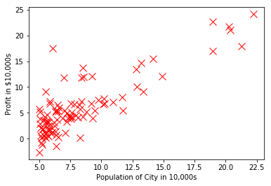
===================== Part 2: Plotting =====================
print('Plotting Data ...')
import pandas as pd
data = pd.read_csv('ex1data1.txt', header=None)
X = data.iloc[:, 0]
y = data.iloc[:, 1]
m = len(y) # number of training examples

# Plot Data
plotData(np.array(X), np.array(y))
Plotting Data ...
============= Part 3: Cost and Gradient descent =============
代价函数
\[J(\theta) = \frac{1}{2m}\sum_{i=1}^{m}{\left(h_\theta(x^{(i)}) - y^{(i)}\right)^2} = \frac{1}{2m}\left((X\theta - y)^T(X\theta - y)\right)\]X = pd.DataFrame(data.iloc[:, 0])
X.insert(0, None, 1) # Add a column of ones to x
X = np.array(X)
y = np.array(y)
theta = np.zeros(2) # initialize fitting parameters
# Some gradient descent settings
iterations = 1500
alpha = 0.01
print('Testing the cost function ...')
# compute and display initial cost
J = computeCost(X, y, theta)
print(f'With theta = [0 ; 0]\nCost computed = {J:f}')
print('Expected cost value (approx) 32.07')
# further testing of the cost function
J = computeCost(X, y, np.array([-1, 2]))
print(f'\nWith theta = [-1 ; 2]\nCost computed = {J:f}')
print('Expected cost value (approx) 54.24')
Testing the cost function ...
With theta = [0 ; 0]
Cost computed = 32.072734
Expected cost value (approx) 32.07

With theta = [-1 ; 2]
Cost computed = 54.242455
Expected cost value (approx) 54.24
梯度下降
\[\theta_j = \theta_j - \alpha\frac{\partial}{\partial\theta_j}J(\theta) = \theta_j - \alpha\frac{1}{m}\sum_{i=1}^{m}\left(h_\theta(x^{(i)}) - y^{(i)}\right)\cdot x_j^{(i)} = \theta_j - \alpha\frac{1}{m}(X\theta - y)^TX_j\] \[\theta = \theta - \alpha\frac{1}{m}\left(X^T(X\theta - y)\right)\]print('Running Gradient Descent ...')
# run gradient descent
theta, J_history = gradientDescent(X, y, theta, alpha, iterations)
# print theta to screen
print(f'Theta found by gradient descent:\n{theta}');
print('Expected theta values (approx)\n -3.6303\n 1.1664\n');
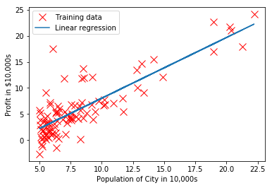
# Plot the linear fit
plotData(X[:, 1], y) # keep previous plot visible
plt.plot(X[:, 1], np.matmul(X, theta), '-')
plt.legend(['Training data', 'Linear regression'])
plt.show() # don't overlay any more plots on this figure
# Predict values for population sizes of 35,000 and 70,000
predict1 = np.matmul(np.array([1, 3.5]), theta)
print(f'For population = 35,000, we predict a profit of {predict1*10000:f}')
predict2 = np.matmul(np.array([1, 7]), theta)
print(f'For population = 70,000, we predict a profit of {predict2*10000:f}')
Running Gradient Descent ...
Theta found by gradient descent:
[-3.630291  1.166362]
Expected theta values (approx)
 -3.6303
  1.1664
For population = 35,000, we predict a profit of 4519.767868
For population = 70,000, we predict a profit of 45342.450129
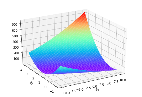
============= Part 4: Visualizing J(\(\theta_0\), \(\theta_1\)) =============
print('Visualizing J(theta_0, theta_1) ...')
# Grid over which we will calculate J
theta0_vals = np.linspace(-10, 10, 100)
theta1_vals = np.linspace(-1, 4, 100)
# initialize J_vals to a matrix of 0's
J_vals = np.zeros((len(theta0_vals), len(theta1_vals)));
# Fill out J_vals
for i in range(len(theta0_vals)):
for j in range(len(theta1_vals)):
t = np.array([theta0_vals[i], theta1_vals[j]])
J_vals[i, j] = computeCost(X, y, t)
# Because of the way meshgrids work in the surf command, we need to
# transpose J_vals before calling surf, or else the axes will be flipped
theta0_vals, theta1_vals = np.meshgrid(theta0_vals, theta1_vals)
J_vals = J_vals.transpose()
# Surface plot
from mpl_toolkits.mplot3d import Axes3D
ax = Axes3D(plt.figure())
ax.view_init(azim=-120)
ax.plot_surface(theta0_vals, theta1_vals, J_vals, cmap='rainbow')
plt.xlabel(r'$\theta_0$')
plt.ylabel(r'$\theta_1$')
plt.show()
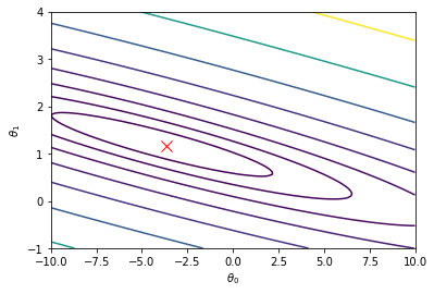
# Contour plot
# Plot J_vals as 15 contours spaced logarithmically between 0.01 and 100
plt.contour(theta0_vals, theta1_vals, J_vals, np.logspace(-2, 3, 20))
plt.xlabel(r'$\theta_0$')
plt.ylabel(r'$\theta_1$')
plt.plot(theta[0], theta[1], 'rx', MarkerSize=10, LineWidth=2)
plt.show()
Visualizing J(theta_0, theta_1) ...
以上部分函数代码在ex1.py中
Exercise 1: Linear regression with multiple variables
=============== Part 1: Feature Normalization ===============
from ex1_multi import *
print('Loading data ...')

## Load Data
data = pd.read_csv('ex1data2.txt', header=None)
X = data.iloc[:, :2]
y = data.iloc[:, 2]

# Print out some data points
print('First 10 examples from the dataset: ')
for i in range(10):
    print(f' x = [{X.iloc[i, 0]} {X.iloc[i, 1]}], y = {y.iloc[i]} ')
Loading data ...
First 10 examples from the dataset:
 x = [2104 3], y = 399900
 x = [1600 3], y = 329900
 x = [2400 3], y = 369000
 x = [1416 2], y = 232000
 x = [3000 4], y = 539900
 x = [1985 4], y = 299900
 x = [1534 3], y = 314900
 x = [1427 3], y = 198999
 x = [1380 3], y = 212000
 x = [1494 3], y = 242500
# Scale features and set them to zero mean
print('Normalizing Features ...')

X, mu, sigma = featureNormalize(X)

# Add intercept term to X
X.insert(0, None, 1)
Normalizing Features ...
================ Part 2: Gradient Descent ================
gradientDescentMulti和computeCostMulti方法跟单变量的一模一样,因为已经实现了通用性
print('Running gradient descent ...');

# Choose some alpha value
alpha = 0.01
num_iters = 400

# Init Theta and Run Gradient Descent
X = np.array(X)
y = np.array(y)
theta = np.zeros(3)
theta, J_history = gradientDescentMulti(X, y, theta, alpha, num_iters)

# Plot the convergence graph
from matplotlib import pyplot as plt
plt.plot(np.arange(num_iters), J_history, '-b', LineWidth=2)
plt.xlabel('Number of iterations')
plt.ylabel('Cost J')
plt.show()

# Display gradient descent's result
print('Theta computed from gradient descent: ');
print(f' {theta} ');
Running gradient descent ...
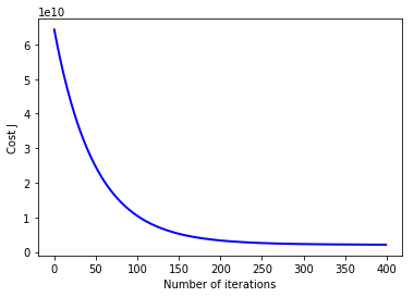
Theta computed from gradient descent:
 [334302.063993  99411.449474   3267.012854]
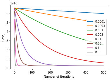
Selecting learning rates
learning_rates = sorted(np.hstack((np.logspace(-4, -1, 4), 3 * np.logspace(-4, -1, 4))))
num_iters = 500
for alpha in learning_rates:
    theta = np.zeros(3)
    theta, J_history = gradientDescentMulti(X, y, theta, alpha, num_iters)
    plt.plot(np.arange(num_iters), J_history, '-', LineWidth=2)
plt.xlabel('Number of iterations')
plt.ylabel('Cost J')
plt.legend([f'{x:.6g}' for x in learning_rates], loc='right')
plt.show()
# Choose some alpha value
alpha = 0.03
num_iters = 400

# Init Theta and Run Gradient Descent
X = np.array(X)
y = np.array(y)
theta = np.zeros(3)
theta, J_history = gradientDescentMulti(X, y, theta, alpha, num_iters)

# Estimate the price of a 1650 sq-ft, 3 br house
house = np.array([1, (1650 - mu[0]) / sigma[0], (3 - mu[1]) / sigma[1]])
price = np.matmul(theta, house)


# ============================================================

print(f'Predicted price of a 1650 sq-ft, 3 br house (using gradient descent):\n ${price:f}')
Predicted price of a 1650 sq-ft, 3 br house (using gradient descent):
 $293142.433485
================ Part 3: Normal Equations ================
正规方程的解
\[\theta = \left(X^TX\right)^{-1}X^Ty\]## Load Data
data = pd.read_csv('ex1data2.txt', header=None)
X = data.iloc[:, :2]
y = data.iloc[:, 2]
m = len(y)
# Add intercept term to X
X.insert(0, None, 1)
# Calculate the parameters from the normal equation
X = np.array(X)
y = np.array(y)
theta = normalEqn(X, y)
# Display normal equation's result
print('Theta computed from the normal equations: ')
print(f' {theta} \n')
# Estimate the price of a 1650 sq-ft, 3 br house
house = np.array([1, 1650, 3])
price = np.matmul(theta, house)
# ============================================================
print(f'Predicted price of a 1650 sq-ft, 3 br house (using normal equations):\n ${price:f}')
Theta computed from the normal equations:
 [89597.909543   139.210674 -8738.019112]

Predicted price of a 1650 sq-ft, 3 br house (using normal equations):
 $293081.464335
两种方法的预测结果还是比较相近的。